CMU Randomized Algorithms
Randomized Algorithms, Carnegie Mellon: Spring 2011
Final exam
on the webpage, or here. Good luck!
Update: Remember it’s due 48 hours after you start, or Friday May 6, 11:59pm, whichever comes first.
Fixes: 1(b): “feasible solution to the LP plus the odd cycle inequalities.” And you need to only show the value is 
FCEs, Final, etc.
Thanks for the great presentations yesterday, everyone!
The final will be posted on the course webpage Friday 4/29 evening at the latest, I will post something on the blog once we’ve done so. You can take it in any contiguous 48 hour period of your choice — just download it when you are ready, and hand in your solutions within 48 hours of that. Slip it under my door (preferably), or email it to me otherwise. We’ll stop accepting solutions at 11:59pm on Friday 5/6.
The course FCEs are now online: please give us your feedback!!
Karger’s min-cut algorithm
Hey, it may be useful for today’s lecture if you have a quick read over Karger’s randomized algorithm for min-cuts. Just the basic algorithm and analysis—we won’t need the improved Karger-Stein variant.
HW #6 Open Thread
HW#6 is out, it’s a short one. Due next Wednesday April 27th.
Lecture 21: Random walks on graphs
Today we talked about random walks on graphs, and the result that in any connected undirected graph G, for any given start vertex u, the expected time for a random walk to visit all the nodes of G (called the cover time of the graph) is at most 2m(n-1), where n is the number of vertices of G and m is the number of edges.
In the process, we proved that for any G, if we think of the walk as at any point in time being on some edge heading in some direction, then each edge/direction is equally likely at probability 1/(2m) at the stationary distribution. (Actually, since we didn’t need to, we didn’t prove it is unique. However, if G is connected, it is not hard to prove by contradiction that there is a unique stationary distribution). We then used that to prove that the expected gap between successive visits to any given (u,v) is 2m. See the notes.
We also gave a few examples to show this is existentially tight. For instance, on a line (n vertices, n-1 edges) we have an expected 

We ended our discussion by talking about resistive networks, and using the connection to give another proof of the cover time of a graph. In particular, we have 


Lecture #20: Rademacher bounds
In this lecture we talked about Rademacher bounds in machine learning. These are never worse and sometimes can be quite a bit tighter than VC-dimension bounds. Rademacher bounds say that to bound how much you are overfitting (the gap between your error on the training set and your true error on the distribution), you can do the following. See how much you would overfit on random labels (how much better than 50% is the empirical error of the best function in your class when you give random labels to your dataset) and then double that quantity (and add a low-order term). See the notes.
HW #5 Open Thread
HW5 has been posted; it’s due on Monday April 4th.
Update: for Exercise #2, the expression ![E_{T \gets \mathcal{D}} [\max_{v \in V} d(v, F_T)]](https://s0.wp.com/latex.php?latex=E_%7BT+%5Cgets+%5Cmathcal%7BD%7D%7D+%5B%5Cmax_%7Bv+%5Cin+V%7D+d%28v%2C+F_T%29%5D&bg=f7f7f7&fg=242424&s=0&c=20201002)


A simpler problem, if you’re stuck, is the furthest pair problem. Here, you are given a metric and want to output a pair of points whose distance is the largest. A natural (yet lousy) algorithm would be: embed the metric into a random tree while maintaining distances in expectation, find a furthest pair in the tree, and output this pair. Show an example where this algorithm sucks.
Lecture #19: Martingales
1. Some definitions
Recall that a martingale is a sequence of r.v.s 


![{E[|Z_i|] < \infty}](https://s0.wp.com/latex.php?latex=%7BE%5B%7CZ_i%7C%5D+%3C+%5Cinfty%7D&bg=f7f7f7&fg=000000&s=0&c=20201002)
![\displaystyle E[Z_i \mid Z_0,...,Z_{i-1}] = Z_{i-1}.](https://s0.wp.com/latex.php?latex=%5Cdisplaystyle++E%5BZ_i+%5Cmid+Z_0%2C...%2CZ_%7Bi-1%7D%5D+%3D+Z_%7Bi-1%7D.+&bg=f7f7f7&fg=000000&s=0&c=20201002)
Somewhat more generally, given a sequence 
-
- there exists functions
such that
, and
-
.
One can define things even more generally, but for the purposes of this course, let’s just proceed with this. If you’d like more details, check out, say, books by Grimmett and Stirzaker, or Durett, or many others.)
1.1. The Azuma-Hoeffding Inequality
Theorem 1 (Azuma-Hoeffding) If
,
. Then
![\displaystyle \Pr[|Z_n - Z_0| \geq \lambda] \leq 2\exp\left\{-\frac{\lambda^2}{2 \sum_i c_i^2} \right\}.](https://s0.wp.com/latex.php?latex=%5Cdisplaystyle++%5CPr%5B%7CZ_n+-+Z_0%7C+%5Cgeq+%5Clambda%5D+%5Cleq+2%5Cexp%5Cleft%5C%7B-%5Cfrac%7B%5Clambda%5E2%7D%7B2+%5Csum_i+c_i%5E2%7D+%5Cright%5C%7D.+&bg=f7f7f7&fg=000000&s=0&c=20201002)
(Apparently Bernstein had essentially figured this one out as well, in addition to the Chernoff-Hoeffding bounds, back in 1937.) The proof of this bound can be found in most texts, we’ll skip it here. BTW, if you just want the upper or lower tail, replace 

2. The Doob Martingale
Most often, the case we will be concerned with is where our entire space is defined by a sequence of random variables 


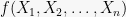
How concentrated is
around its mean
?
To this end, define for every 
![\displaystyle Z_i := E[ f(X) \mid X_1, X_2, \ldots,X_i ].](https://s0.wp.com/latex.php?latex=%5Cdisplaystyle++Z_i+%3A%3D+E%5B+f%28X%29+%5Cmid+X_1%2C+X_2%2C+%5Cldots%2CX_i+%5D.+&bg=f7f7f7&fg=000000&s=0&c=20201002)
(At this point, it is useful to remember the definition of a random variable as a function from the sample space to the reals: so this r.v.
How does the random variable 
![{E[f]}](https://s0.wp.com/latex.php?latex=%7BE%5Bf%5D%7D&bg=f7f7f7&fg=000000&s=0&c=20201002)


![{Z_1(x_1) = E_{X_2, \ldots, X_n}[f(x_1, X_2, \ldots, X_n)]}](https://s0.wp.com/latex.php?latex=%7BZ_1%28x_1%29+%3D+E_%7BX_2%2C+%5Cldots%2C+X_n%7D%5Bf%28x_1%2C+X_2%2C+%5Cldots%2C+X_n%29%5D%7D&bg=f7f7f7&fg=000000&s=0&c=20201002)


Of course, we’re defining this for a reason:
Lemma 2 For a bounded function
is a martingale with respect to
Proof: The first two properties of
![\displaystyle \begin{array}{rl} E[Z_i \mid X_1, \ldots X_{i-1}] &= E[\, E[f \mid X_1, X_2, \ldots, X_i] \mid X_1, \ldots X_{i-1} ] \\ &= E[ f \mid X_1, \ldots X_{i-1} ] = Z_{i-1}. \end{array}](https://s0.wp.com/latex.php?latex=%5Cdisplaystyle++%5Cbegin%7Barray%7D%7Brl%7D++E%5BZ_i+%5Cmid+X_1%2C+%5Cldots+X_%7Bi-1%7D%5D+%26%3D+E%5B%5C%2C+E%5Bf+%5Cmid+X_1%2C+X_2%2C+%5Cldots%2C+X_i%5D+%5Cmid+X_1%2C+%5Cldots+X_%7Bi-1%7D+%5D+%5C%5C+%26%3D+E%5B+f+%5Cmid+X_1%2C+%5Cldots+X_%7Bi-1%7D+%5D+%3D+Z_%7Bi-1%7D.+%5Cend%7Barray%7D+&bg=f7f7f7&fg=000000&s=0&c=20201002)
The first equaility is the definition of ![{E[ U \mid V ] = E[ E[ U \mid V, W ] \mid V ]}](https://s0.wp.com/latex.php?latex=%7BE%5B+U+%5Cmid+V+%5D+%3D+E%5B+E%5B+U+%5Cmid+V%2C+W+%5D+%5Cmid+V+%5D%7D&bg=f7f7f7&fg=000000&s=0&c=20201002)


Assuming that
Before we continue on this thread, let us show some Doob martingales which arise in CS/Math-y applications.
- Throw
balls into
, and
,
- Consider the random graph
:
edges chosen independently with probability
. Let
be the chromatic number of the graph, the minimum number of colors to properly color the graph. There are two natural Doob martingales associated with this, depending on how we choose the variables
In the first one, let
edge, and which gives us a martingle sequence of length
: the new martingale has length
- Consider a run of quicksort on a particular input: let
be the number of comparisons. Let
the second, etc. Then
is a Doob martingale with respect to
BTW, are these
and use that to pick a random element from the current set, etc.)
- Suppose we have
red and
blue balls in a bin. We draw
is the number of red balls. Then
However, in this example, the
So yeah, if we want to study the concentration of
Next step: to apply Azuma-Hoeffding to the Doob martingale 


2.1. Indepedence and Lipschitz-ness
One case when it’s easy to bound the
Definition 3 Given values
, the function
-Lipschitz} if for all
and
, for all
and for all
, it holds that
If
for all
-Lipschitz.

Lemma 4 If

Proof: Let us use 

![\displaystyle \begin{array}{rl} Z_i &= E[ f \mid X_{(1:i)} ] = \sum_{a_{i+1}, \ldots, a_n} f(X_{(1:i)}, a_{(i+1:n)}) \Pr[ X_{(i+1:n)} = a_{(i+1:n)} \mid X_{(1:i)} ] \\ &= \sum_{a_{i+1}, \ldots, a_n} f(X_{(1:i)}, a_{(i+1:n)}) \Pr[ X_{(i+1:n)} = a_{(i+1:n)} ] \end{array}](https://s0.wp.com/latex.php?latex=%5Cdisplaystyle++%5Cbegin%7Barray%7D%7Brl%7D++Z_i+%26%3D+E%5B+f+%5Cmid+X_%7B%281%3Ai%29%7D+%5D+%3D+%5Csum_%7Ba_%7Bi%2B1%7D%2C+%5Cldots%2C+a_n%7D+f%28X_%7B%281%3Ai%29%7D%2C+a_%7B%28i%2B1%3An%29%7D%29+%5CPr%5B+X_%7B%28i%2B1%3An%29%7D+%3D+a_%7B%28i%2B1%3An%29%7D+%5Cmid+X_%7B%281%3Ai%29%7D+%5D+%5C%5C+%26%3D+%5Csum_%7Ba_%7Bi%2B1%7D%2C+%5Cldots%2C+a_n%7D+f%28X_%7B%281%3Ai%29%7D%2C+a_%7B%28i%2B1%3An%29%7D%29+%5CPr%5B+X_%7B%28i%2B1%3An%29%7D+%3D+a_%7B%28i%2B1%3An%29%7D+%5D+%5Cend%7Barray%7D+&bg=f7f7f7&fg=000000&s=0&c=20201002)
where the last equality is from independence. Similarly for
![\displaystyle \begin{array}{rl} | Z_i - Z_{i-1} | &= \sum_{a_{i+1}, \ldots, a_n} \bigg| f(X_{(1:i)}, a_{(i+1:n)}) - \sum_{a_i'} \Pr[X_i = a_i'] f(X_{(1:i-1)}, a_i', a_{(i+1:n)}) \bigg| \cdot \Pr[ X_{(i+1:n)} = a_{(i+1:n)} ] \\ &\le \sum_{a_{i+1}, \ldots, a_n} c_i \cdot \Pr[ X_{(i+1:n)} = a_{(i+1:n)} ] = c_i. \end{array}](https://s0.wp.com/latex.php?latex=%5Cdisplaystyle++%5Cbegin%7Barray%7D%7Brl%7D++%7C+Z_i+-+Z_%7Bi-1%7D+%7C+%26%3D+%5Csum_%7Ba_%7Bi%2B1%7D%2C+%5Cldots%2C+a_n%7D+%5Cbigg%7C+f%28X_%7B%281%3Ai%29%7D%2C+a_%7B%28i%2B1%3An%29%7D%29+-+%5Csum_%7Ba_i%27%7D+%5CPr%5BX_i+%3D+a_i%27%5D+f%28X_%7B%281%3Ai-1%29%7D%2C+a_i%27%2C+a_%7B%28i%2B1%3An%29%7D%29+%5Cbigg%7C+%5Ccdot+%5CPr%5B+X_%7B%28i%2B1%3An%29%7D+%3D+a_%7B%28i%2B1%3An%29%7D+%5D+%5C%5C+%26%5Cle+%5Csum_%7Ba_%7Bi%2B1%7D%2C+%5Cldots%2C+a_n%7D+c_i+%5Ccdot+%5CPr%5B+X_%7B%28i%2B1%3An%29%7D+%3D+a_%7B%28i%2B1%3An%29%7D+%5D+%3D+c_i.+%5Cend%7Barray%7D+&bg=f7f7f7&fg=000000&s=0&c=20201002)
where the inequality is from the fact that changing the 


![{\sum_{a_i'} \Pr[X_i = a_i'] = 1}](https://s0.wp.com/latex.php?latex=%7B%5Csum_%7Ba_i%27%7D+%5CPr%5BX_i+%3D+a_i%27%5D+%3D+1%7D&bg=f7f7f7&fg=000000&s=0&c=20201002)
Now applying Azuma-Hoeffding, we immediately get:
Corollary 5 (McDiarmid’s Inequality) If
is
![\displaystyle \begin{array}{rl} \Pr[ f - E[f] \geq \lambda ] &\leq \exp\left( - \frac{ \lambda^2 }{2 \sum_i c_i^2 } \right), \\ \Pr[ f - E[f] < \lambda ] &\leq \exp\left( - \frac{ \lambda^2 }{2 \sum_i c_i^2 } \right). \end{array}](https://s0.wp.com/latex.php?latex=%5Cdisplaystyle++%5Cbegin%7Barray%7D%7Brl%7D++%5CPr%5B+f+-+E%5Bf%5D+%5Cgeq+%5Clambda+%5D+%26%5Cleq+%5Cexp%5Cleft%28+-+%5Cfrac%7B+%5Clambda%5E2+%7D%7B2+%5Csum_i+c_i%5E2+%7D+%5Cright%29%2C+%5C%5C+%5CPr%5B+f+-+E%5Bf%5D+%3C+%5Clambda+%5D+%26%5Cleq+%5Cexp%5Cleft%28+-+%5Cfrac%7B+%5Clambda%5E2+%7D%7B2+%5Csum_i+c_i%5E2+%7D+%5Cright%29.+%5Cend%7Barray%7D+&bg=f7f7f7&fg=000000&s=0&c=20201002)
(Disclosure: I am cheating. McDiarmid’s inequality has better constants, the constant 
- For the
. Also, changing the location of the
. So
Hence, whp,
.
- For the case where
, clearly
This is not very interesting, since the right hand side is
only when
—but the chromatic number itself lies in
, so we get almost no concentration at all.
Instead, we could use a vertex-exposure martingale, where at the
And hence the chromatic number of the random graph
around its mean.
![\displaystyle \Pr [ | f - Ef | \geq \lambda ] \leq 2 \exp\left( - \frac{\lambda^2}{2m} \right).](https://s0.wp.com/latex.php?latex=%5Cdisplaystyle++%5CPr+%5B+%7C+f+-+Ef+%7C+%5Cgeq+%5Clambda+%5D+%5Cleq+2+%5Cexp%5Cleft%28+-+%5Cfrac%7B%5Clambda%5E2%7D%7B2m%7D+%5Cright%29.+&bg=f7f7f7&fg=000000&s=0&c=20201002)
![\displaystyle \Pr [ | \chi - E\chi | \geq \lambda ] \leq 2 \exp\left( - \frac{\lambda^2}{2\binom{n}{2}} \right)](https://s0.wp.com/latex.php?latex=%5Cdisplaystyle++%5CPr+%5B+%7C+%5Cchi+-+E%5Cchi+%7C+%5Cgeq+%5Clambda+%5D+%5Cleq+2+%5Cexp%5Cleft%28+-+%5Cfrac%7B%5Clambda%5E2%7D%7B2%5Cbinom%7Bn%7D%7B2%7D%7D+%5Cright%29+&bg=f7f7f7&fg=000000&s=0&c=20201002)
![\displaystyle \Pr [ | \chi - E\chi | \geq \lambda ] \leq 2 \exp\left( - \frac{\lambda^2}{2n} \right)](https://s0.wp.com/latex.php?latex=%5Cdisplaystyle++%5CPr+%5B+%7C+%5Cchi+-+E%5Cchi+%7C+%5Cgeq+%5Clambda+%5D+%5Cleq+2+%5Cexp%5Cleft%28+-+%5Cfrac%7B%5Clambda%5E2%7D%7B2n%7D+%5Cright%29&bg=f7f7f7&fg=000000&s=0&c=20201002)
3. Concentration for Random Geometric TSP
McDiarmid’s inequality is convenient to use, but Lipschitz-ness often does not get us as far as we’d like (even with independence). Sometimes you need to bound
Let
. Let
be the length of the shortest traveling salesman tour on
concentrated around its mean
?
In the HW, you will show that 

3.1. Using McDiarmid: a weak first bound
Note that 
![\displaystyle \Pr[ |\tau - E\tau| \geq \lambda ] \leq 2 \exp( -\frac{\lambda^2}{16n}).](https://s0.wp.com/latex.php?latex=%5Cdisplaystyle++%5CPr%5B+%7C%5Ctau+-+E%5Ctau%7C+%5Cgeq+%5Clambda+%5D+%5Cleq+2+%5Cexp%28+-%5Cfrac%7B%5Clambda%5E2%7D%7B16n%7D%29.+&bg=f7f7f7&fg=000000&s=0&c=20201002)
If we want the deviation probability to be 

3.2. So let’s be more careful: an improved bound
And in fact, we’ll get a better bound using the very same Doob martingale
![\displaystyle Z_i = E[ \tau(X_1, X_2, \ldots, X_n) \mid X_1, X_2, \ldots, X_i ].](https://s0.wp.com/latex.php?latex=%5Cdisplaystyle++Z_i+%3D+E%5B+%5Ctau%28X_1%2C+X_2%2C+%5Cldots%2C+X_n%29+%5Cmid+X_1%2C+X_2%2C+%5Cldots%2C+X_i+%5D.+&bg=f7f7f7&fg=000000&s=0&c=20201002)
But instead of just using the 
Before we prove this lemma, let us complete the concentration bound for TSP using this. Setting 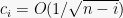
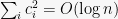
![\displaystyle \Pr[ |\tau - E\tau| \geq \lambda ] \leq 2 \exp\left( -\frac{\lambda^2}{2\sum_{i} c_i^2}\right) \leq 2 \exp\left( - \frac{\lambda^2}{O(\log n)} \right).](https://s0.wp.com/latex.php?latex=%5Cdisplaystyle++%5CPr%5B+%7C%5Ctau+-+E%5Ctau%7C+%5Cgeq+%5Clambda+%5D+%5Cleq+2+%5Cexp%5Cleft%28+-%5Cfrac%7B%5Clambda%5E2%7D%7B2%5Csum_%7Bi%7D+c_i%5E2%7D%5Cright%29+%5Cleq+2+%5Cexp%5Cleft%28+-+%5Cfrac%7B%5Clambda%5E2%7D%7BO%28%5Clog+n%29%7D+%5Cright%29.+&bg=f7f7f7&fg=000000&s=0&c=20201002)
So
![\displaystyle \Pr[ | \tau - E\tau | \leq O(\log n) ] \geq 1 - 1/poly(n).](https://s0.wp.com/latex.php?latex=%5Cdisplaystyle++%5CPr%5B+%7C+%5Ctau+-+E%5Ctau+%7C+%5Cleq+O%28%5Clog+n%29+%5D+%5Cgeq+1+-+1%2Fpoly%28n%29.+&bg=f7f7f7&fg=000000&s=0&c=20201002)
Much better!
3.3. Some useful lemmas
To prove Lemma 6, we’ll need a simple geometric lemma:
Lemma 7 Let
. Pick
random points
from
to its closest point in
.
Proof: Define the random variable 


![{r \in [0,\sqrt{2}]}](https://s0.wp.com/latex.php?latex=%7Br+%5Cin+%5B0%2C%5Csqrt%7B2%7D%5D%7D&bg=f7f7f7&fg=000000&s=0&c=20201002)
![{B(x, r) \cap [0,1]^2}](https://s0.wp.com/latex.php?latex=%7BB%28x%2C+r%29+%5Ccap+%5B0%2C1%5D%5E2%7D&bg=f7f7f7&fg=000000&s=0&c=20201002)


Define 
![{r = \lambda r_0 \in [0,\sqrt{2}]}](https://s0.wp.com/latex.php?latex=%7Br+%3D+%5Clambda+r_0+%5Cin+%5B0%2C%5Csqrt%7B2%7D%5D%7D&bg=f7f7f7&fg=000000&s=0&c=20201002)
![{\Pr[ W \geq r = \lambda r_0 ]}](https://s0.wp.com/latex.php?latex=%7B%5CPr%5B+W+%5Cgeq+r+%3D+%5Clambda+r_0+%5D%7D&bg=f7f7f7&fg=000000&s=0&c=20201002)

Of course, for 
![{\Pr[W \geq r ] = 0}](https://s0.wp.com/latex.php?latex=%7B%5CPr%5BW+%5Cgeq+r+%5D+%3D+0%7D&bg=f7f7f7&fg=000000&s=0&c=20201002)
![\displaystyle E[W] = \int_{r \geq 0} \Pr[ W \geq r ] dr = \sum_{\lambda \in {\mathbb Z}_{\geq 0}} \int_{r \in [\lambda r_0, (\lambda+1)r_0]} \Pr[ W \geq r ] dr \leq \sum_{\lambda \in {\mathbb Z}_{\geq 0}} (\lambda+1)r_0 \cdot e^{-\lambda^2} \leq O(r_0).](https://s0.wp.com/latex.php?latex=%5Cdisplaystyle++E%5BW%5D+%3D+%5Cint_%7Br+%5Cgeq+0%7D+%5CPr%5B+W+%5Cgeq+r+%5D+dr+%3D+%5Csum_%7B%5Clambda+%5Cin+%7B%5Cmathbb+Z%7D_%7B%5Cgeq+0%7D%7D+%5Cint_%7Br+%5Cin+%5B%5Clambda+r_0%2C+%28%5Clambda%2B1%29r_0%5D%7D+%5CPr%5B+W+%5Cgeq+r+%5D+dr+%5Cleq+%5Csum_%7B%5Clambda+%5Cin+%7B%5Cmathbb+Z%7D_%7B%5Cgeq+0%7D%7D+%28%5Clambda%2B1%29r_0+%5Ccdot+e%5E%7B-%5Clambda%5E2%7D+%5Cleq+O%28r_0%29.+&bg=f7f7f7&fg=000000&s=0&c=20201002)
Secondly, here is another lemma about how the TSP behaves:
Lemma 8 For any set of
points,
, we get

Proof: Follows from the fact that ![{\tau(A + x) \in [TSP(A), TSP(A) + 2d(x, A)]}](https://s0.wp.com/latex.php?latex=%7B%5Ctau%28A+%2B+x%29+%5Cin+%5BTSP%28A%29%2C+TSP%28A%29+%2B+2d%28x%2C+A%29%5D%7D&bg=f7f7f7&fg=000000&s=0&c=20201002)
3.4. Proving Lemma \ref
}
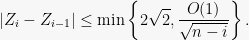
OK, now to the proof of Lemma 6. Recall that we want to bound 

![\displaystyle \begin{array}{rl} Z_{i-1} &= E[ \tau(X_1, X_2, \ldots, X_{i-1}, X_i, \ldots, X_n) \mid X_1, X_2, \ldots, X_{i-1} ] \\ &= E[ \tau(X_1, X_2, \ldots, X_{i-1}, \widehat{X}_i, \ldots, X_n) \mid X_1, X_2, \ldots, X_{i-1} ] \\ &= E[ \tau(X_1, X_2, \ldots, X_{i-1}, \widehat{X}_i, \ldots, X_n) \mid X_1, X_2, \ldots, X_{i} ] \end{array}](https://s0.wp.com/latex.php?latex=%5Cdisplaystyle++%5Cbegin%7Barray%7D%7Brl%7D++Z_%7Bi-1%7D+%26%3D+E%5B+%5Ctau%28X_1%2C+X_2%2C+%5Cldots%2C+X_%7Bi-1%7D%2C+X_i%2C+%5Cldots%2C+X_n%29+%5Cmid+X_1%2C+X_2%2C+%5Cldots%2C+X_%7Bi-1%7D+%5D+%5C%5C+%26%3D+E%5B+%5Ctau%28X_1%2C+X_2%2C+%5Cldots%2C+X_%7Bi-1%7D%2C+%5Cwidehat%7BX%7D_i%2C+%5Cldots%2C+X_n%29+%5Cmid+X_1%2C+X_2%2C+%5Cldots%2C+X_%7Bi-1%7D+%5D+%5C%5C+%26%3D+E%5B+%5Ctau%28X_1%2C+X_2%2C+%5Cldots%2C+X_%7Bi-1%7D%2C+%5Cwidehat%7BX%7D_i%2C+%5Cldots%2C+X_n%29+%5Cmid+X_1%2C+X_2%2C+%5Cldots%2C+X_%7Bi%7D+%5D+%5Cend%7Barray%7D+&bg=f7f7f7&fg=000000&s=0&c=20201002)
where 
![\displaystyle |Z_i - Z_{i-1}| = E[ \tau(X_1, \ldots, X_{i-1}, X_i, \ldots, X_n) - \tau(X_1, \ldots, X_{i-1}, \widehat{X}_i, \ldots, X_n) \mid X_1, X_2, \ldots, X_{i} ].](https://s0.wp.com/latex.php?latex=%5Cdisplaystyle++%7CZ_i+-+Z_%7Bi-1%7D%7C+%3D+E%5B+%5Ctau%28X_1%2C+%5Cldots%2C+X_%7Bi-1%7D%2C+X_i%2C+%5Cldots%2C+X_n%29+-+%5Ctau%28X_1%2C+%5Cldots%2C+X_%7Bi-1%7D%2C+%5Cwidehat%7BX%7D_i%2C+%5Cldots%2C+X_n%29+%5Cmid+X_1%2C+X_2%2C+%5Cldots%2C+X_%7Bi%7D+%5D.+&bg=f7f7f7&fg=000000&s=0&c=20201002)
Then, if we define the set 
![\displaystyle \begin{array}{rl} |Z_i - Z_{i-1}| &= E[ TSP(S \cup T \cup \{X_i\}) - TSP(S \cup T \cup \{\widehat{X}_i\}) \mid X_1, X_2, \ldots, X_{i} ] \\ &\leq E[ 2( d(X_i, S\cup T) + d(\widehat{X}_i, S\cup T)) \mid X_1, X_2, \ldots, X_{i} ] \\ &\leq E_{\widehat{X}_i, T}[ 2( d(X_i, T) + d(\widehat{X}_i, T)) \mid X_{i} ]. \end{array}](https://s0.wp.com/latex.php?latex=%5Cdisplaystyle++%5Cbegin%7Barray%7D%7Brl%7D++%7CZ_i+-+Z_%7Bi-1%7D%7C+%26%3D+E%5B+TSP%28S+%5Ccup+T+%5Ccup+%5C%7BX_i%5C%7D%29+-+TSP%28S+%5Ccup+T+%5Ccup+%5C%7B%5Cwidehat%7BX%7D_i%5C%7D%29+%5Cmid+X_1%2C+X_2%2C+%5Cldots%2C+X_%7Bi%7D+%5D+%5C%5C+%26%5Cleq+E%5B+2%28+d%28X_i%2C+S%5Ccup+T%29+%2B+d%28%5Cwidehat%7BX%7D_i%2C+S%5Ccup+T%29%29+%5Cmid+X_1%2C+X_2%2C+%5Cldots%2C+X_%7Bi%7D+%5D+%5C%5C+%26%5Cleq+E_%7B%5Cwidehat%7BX%7D_i%2C+T%7D%5B+2%28+d%28X_i%2C+T%29+%2B+d%28%5Cwidehat%7BX%7D_i%2C+T%29%29+%5Cmid+X_%7Bi%7D+%5D.+%5Cend%7Barray%7D+&bg=f7f7f7&fg=000000&s=0&c=20201002)
where the first inequality uses Lemma 8 and the second uses the fact that the minimum distance to a set only increses when the set gets smaller. But now we can invoke Lemma 7 to bound each of the terms by 
3.5. Some more about Geometric TSP
For constant dimension 
![{[0,1]^d}](https://s0.wp.com/latex.php?latex=%7B%5B0%2C1%5D%5Ed%7D&bg=f7f7f7&fg=000000&s=0&c=20201002)


The result we just proved was by Rhee and Talagrand, but it was not the last result about TSP concentration. Rhee and Talagrand subsequently improved this bound to the TSP has subgaussian tails!
![\displaystyle \Pr[ |\tau - E\tau| \geq \lambda ] \leq ce^{-\lambda^2/O(1)} .](https://s0.wp.com/latex.php?latex=%5Cdisplaystyle++%5CPr%5B+%7C%5Ctau+-+E%5Ctau%7C+%5Cgeq+%5Clambda+%5D+%5Cleq+ce%5E%7B-%5Clambda%5E2%2FO%281%29%7D+.+&bg=f7f7f7&fg=000000&s=0&c=20201002)
We’ll show a proof of this using Talagrand’s inequality, in a later lecture.
If you’re interested in this line of research, here is a survey article by Michael Steele on concentration properties of optimization problems in Euclidean space, and another one by Alan Frieze and Joe Yukich on many aspects of probabilistic TSP.
4. Citations
As mentioned in a previous post, McDiarmid and Hayward use martingales to give extremely strong concentration results for QuickSort . The book by Dubhashi and Panconesi (preliminary version here) sketches this result, and also contains many other examples and extensions of the use of martingales.
Other resources for concentration using martingales: this survey by Colin McDiarmid, or this article by Fan Chung and Linyuan Lu.
Apart from giving us powerful concentration results, martingales and “stopping times” combine to give very surprising and powerful results: see this survey by Yuval Peres at SODA 2010, or these course notes by Yuval and Eyal Lubetzky.
Lecture #18: Oblivious routing on a hypercube
In celebration of Les Valiant’s winning of the Turing award, today we discussed a classic result of his on the problem of oblivious routing on the hypercube. (Valiant, “A scheme for fast parallel communication”, SIAM J. Computing 1982, and Valiant and Brebner, “Universal schemes for parallel communication”, STOC 1981). The high-level idea is that rather than routing immediately to your final destination, go to a random intermediate point first. The analysis is really beautiful — you define the right quantities and it just magically works out nicely. See today’s class notes. We also discussed the Butterfly and Benes networks as well. (See the excellent notes of Satish Rao for more on them).
At the end, we also briefly discussed Martingales: their definition, Azuma’s inequality, and McDiarmid’s inequality (which doesn’t talk about Martingales directly but is very convenient and can be proven using Azuma). The discussion at the end was extremely rushed but the key point was: suppose you have a complicated random variable 


![X_i = E[\phi | z_1, \ldots, z_i]](https://s0.wp.com/latex.php?latex=X_i+%3D+E%5B%5Cphi+%7C+z_1%2C+%5Cldots%2C+z_i%5D&bg=f7f7f7&fg=242424&s=0&c=20201002)


Lecture #17: Dimension reduction (continued)
1. An equivalent view of estimating 
Again, you have a data stream of elements 

![{[D]}](https://s0.wp.com/latex.php?latex=%7B%5BD%5D%7D&bg=f7f7f7&fg=000000&s=0&c=20201002)


Take a (suitably random) hash function
. Maintain counter
, which starts off at zero. Every time an element
. And when queried, we reply with the value
.
Hence, having seen the stream that results in the frequency vector 

![{E[C^2]}](https://s0.wp.com/latex.php?latex=%7BE%5BC%5E2%5D%7D&bg=f7f7f7&fg=000000&s=0&c=20201002)
![\displaystyle E[C^2] = E[ \sum_{i,j} h(i) h(j) x_ix_j ] = \sum_i x_i^2.](https://s0.wp.com/latex.php?latex=%5Cdisplaystyle+++E%5BC%5E2%5D+%3D+E%5B+%5Csum_%7Bi%2Cj%7D+h%28i%29+h%28j%29+x_ix_j+%5D+%3D+%5Csum_i+x_i%5E2.++&bg=f7f7f7&fg=000000&s=0&c=20201002)
And what about the variance? Recall that ![{\mathrm{Var}(C^2) = E[(C^2)^2] - E[C^2]^2}](https://s0.wp.com/latex.php?latex=%7B%5Cmathrm%7BVar%7D%28C%5E2%29+%3D+E%5B%28C%5E2%29%5E2%5D+-+E%5BC%5E2%5D%5E2%7D&bg=f7f7f7&fg=000000&s=0&c=20201002)
![\displaystyle E[(C^2)^2] = E[ \sum_{p,q,r,s} h(p) h(q) h(r) h(s) x_px_qx_rx_s ] = \sum_p x_p^4 + 6\,\sum_{p < q} x_p^2 x_q^2.](https://s0.wp.com/latex.php?latex=%5Cdisplaystyle+++E%5B%28C%5E2%29%5E2%5D+%3D+E%5B+%5Csum_%7Bp%2Cq%2Cr%2Cs%7D+h%28p%29+h%28q%29+h%28r%29+h%28s%29+x_px_qx_rx_s+%5D+%3D+%5Csum_p+x_p%5E4+%2B+6%5C%2C%5Csum_%7Bp+%3C+q%7D+x_p%5E2+x_q%5E2.++&bg=f7f7f7&fg=000000&s=0&c=20201002)
So
![\displaystyle \text{Var}(C^2) = \sum_p x_p^4 + 6\sum_{p < q} x_p^2x_q^2 - (\sum_p x_p^2)^2 = 4 \sum_{p < q} x_p^2x_q^2 \leq 2 E[C^2]^2.](https://s0.wp.com/latex.php?latex=%5Cdisplaystyle++%5Ctext%7BVar%7D%28C%5E2%29+%3D+%5Csum_p+x_p%5E4+%2B+6%5Csum_%7Bp+%3C+q%7D+x_p%5E2x_q%5E2+-+%28%5Csum_p+x_p%5E2%29%5E2+%3D+4+%5Csum_%7Bp+%3C+q%7D+x_p%5E2x_q%5E2+%5Cleq+2+E%5BC%5E2%5D%5E2.+&bg=f7f7f7&fg=000000&s=0&c=20201002)
What does Chebyshev say then?
![\displaystyle \Pr[ | C^2 - E[C^2] | > \epsilon E[C^2] ] \leq \frac{\text{Var}(C^2)}{(\epsilon E[C^2])^2} \leq \frac{2}{\epsilon^2}.](https://s0.wp.com/latex.php?latex=%5Cdisplaystyle++%5CPr%5B+%7C+C%5E2+-+E%5BC%5E2%5D+%7C+%3E+%5Cepsilon+E%5BC%5E2%5D+%5D+%5Cleq+%5Cfrac%7B%5Ctext%7BVar%7D%28C%5E2%29%7D%7B%28%5Cepsilon+E%5BC%5E2%5D%29%5E2%7D+%5Cleq+%5Cfrac%7B2%7D%7B%5Cepsilon%5E2%7D.+&bg=f7f7f7&fg=000000&s=0&c=20201002)
Not that hot: in fact, this is usually more than
But if we take a collection of 


![\displaystyle \Pr[ | \overline{C}^2 - E[\overline{C}^2] | > \epsilon E[\overline{C}^2] ] \leq \frac{\text{Var}(\overline{C}^2)}{(\epsilon E[\overline{C}^2])^2} \leq \frac{2}{k \epsilon^2}.](https://s0.wp.com/latex.php?latex=%5Cdisplaystyle++%5CPr%5B+%7C+%5Coverline%7BC%7D%5E2+-+E%5B%5Coverline%7BC%7D%5E2%5D+%7C+%3E+%5Cepsilon+E%5B%5Coverline%7BC%7D%5E2%5D+%5D+%5Cleq+%5Cfrac%7B%5Ctext%7BVar%7D%28%5Coverline%7BC%7D%5E2%29%7D%7B%28%5Cepsilon+E%5B%5Coverline%7BC%7D%5E2%5D%29%5E2%7D+%5Cleq+%5Cfrac%7B2%7D%7Bk+%5Cepsilon%5E2%7D.+&bg=f7f7f7&fg=000000&s=0&c=20201002)
So, our probability of error on any query is at most 

1.1. Hey, those calculations look familiar
Sure. This is just a restatement of what we did in lecture. There we took a matrix 


1.2. Limited Independence
How much randomness do you need for the hash functions? Indeed, hash functions which are 
